 |
 |
 |
 |
 |
 |
|
The basic amplifierBefore we dig into the many things that one can do with an operational amplifier, I'm just going to do a quick overview of the basic device, and what can be expected of it. For many this information might be unnecessary, but I've put it here anyway. I know that when I was first going through all of this, years ago, the simple basics were not obvious. I could see what was going on with overall functionality, but it was much harder to penetrate the details because I had no clear picture of the basics. In simple circuits op-amps are so nearly ideal components, I think they lend themselves as a starting point in analogue electronics. In structured thinking, and formal training, lessons usually start with the transistor. I'm not entirely sure that's the right way to go. Because Op-Amps are so ideal, and so useful, they lend themselves well to experimentation. They foster interest in learning more about the other components and techniques, to achieve more things.
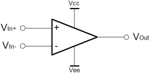
After passive components, learning usually progresses through diodes and transistors. Since it is such a significant leap between a single transistor and a full on differential voltage amplifier this seems slightly odd. An Op-Amp works so simply and well from the outside, I think it better to return to transistors when the ambiguities are less of an affront to the novice mind. I would make the simple comparison, about learning to live in the world, before trying to understand atomic theory. The other way around, we might as well be amoebae, rather than humans. Notwithstanding, this does not make amoebae less important. The diagram on the left depicts the circuit symbol for the Op-Amp. Although it is shown here as a five terminal device, it can be thought of as a three terminal device. The power supply connections, above and below, are often omitted from diagrammatic representations. As a three terminal device, the op-amp is comparable with the apparent simplicity of the transistor. Unlike the transistor, there is no thinking overhead associated with the supply of power to make the component work. Since an Op-Amp has separate supplies, biasing, load-lines, logarithmic behaviours, temperature effects all fall away. One can concentrate on the core principles involved and revisit the complexity of transistors as the desire or need require.
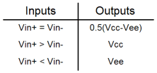
I think that the best way to think about the Op-Amp, in the first instance, is as a logic device. Since many people come to electronics from a programming background, perhaps playing with a computer at weekends, many will probably already be familiar with the idea of a truth table. On the right is the "analogue truth table" for the Op-Amp. It's fuzzy logic. It's the future. One wire can signal more than just a binary level! Whilst there are good reasons for binary systems, sometimes, one has cause to think that analogue was better than digital for a time, and will be better again one day.
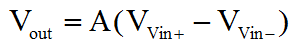
An Op-Amp typically has huge gain. It's not always true, especially for niche high speed amplifiers. Typically these aren't really proper Op-Amps so we'll ignore that. The output is simply the difference of the inputs multiplied by the gain (denoted by A) in the equation on the left. Because the Op-Amp has such large gain, the truth table, above more or less holds true. The difference in voltage between the positive and negative inputs is in the order of millivolts or perhaps microvolts, and yet the output will slew off to the maximum possible extent. The obvious practical problem lies in the first line of the truth table. That line suggests that if the inputs are exactly equal, then the output will be at a level exactly half way between the supply rails. That's not quite true, and is the reason for the logically "fuzzy" behaviour of an Op-Amp. In the "open loop" configuration shown here, it's what one would expect in a perfect world. In practice, it's probably better to think of the output as "floating" in this circumstance.
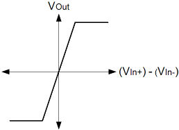
The diagram on the right is a plot of the ideal behaviour of an Op-Amp, to try and put a picture to the truth table. It shows the difference between the inputs horizontally, against the output vertically. Again, this is idealised, but the graph is important, to understanding the basic constraints of the Op-Amp. In practice the slope is much steeper than that shown. As you can perhaps begin to see, the important thing about the Op-Amp is that the output changes very quickly in relation to very small changes in the difference between the inputs. When thinking about Op-Amps, the most important thing to remember is that in the normal "closed loop" configuration, which we'll see shortly, the inputs will usually have more or less the same voltage on them. This will be true, to within a range of just a few millivolts, perhaps even microvolts; except in just a few particular open loop applications. In the closed loop configuration, the inverting input is normally connected in some way to the output. When the difference between inputs is small, the output trends in a direction for a given input stimulus. This is opposed to the idea that the output takes on a particular value. Because one input represents the stimulus now, and the other (by virtue of it's connection to the output) represents the output as a function of what the input was, the output trend can be thought of as some differential of the input, with respect to time, as in the calculus.
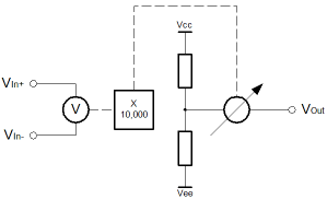
The diagram on the left shows that there is nothing spectacularly complicated inside the ideal Op-Amp. I've already said that things are not quite that simple, but nevertheless, the diagram holds reasonably true, even if the insides of an Op-Amp are actually pretty complicated in the details. The aim is to simplify things, and make them not seem too frightening. It can be complicated if you want, but actually it's pretty simple. The inputs can be thought of as having a voltmeter across them. The output has a perfect resistive divider, which divides the power supply exactly in half. The divider magically divides the supply rails, whilst having zero resistance. Connected to the middle of the divider is one side of a variable voltage source. The other side connects to the output. Between the input and output is some more magic. It simply reads the voltmeter on the input, and multiplies the reading by an arbitrary large number; the gain. Take the new number and set the output voltage as close as possible. In practice the bigger the gain multiplier the better. Sure, the output will usually be saturated if there is almost any difference between the inputs. That's exactly what we want. In practice, the multiplier might be bigger, or smaller. Smaller can cause problems. Usually it's bigger. It is critically significant that the inputs have a high resistance. Little or no current enters the voltmeter, as one would expect. Equally the output resistance is very low, similar (or better) than that which one might expect from a battery. This feature is essential to the high performance of the Op-Amp, and in its use as a true voltage amplifier.
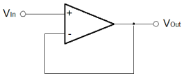
Let's now take a look at the use of an Op-Amp as a unity gain (gain of 1) buffer. By closing the loop in the simplest possible way, we throw away all of the gain that the amplifier has, but we still get a device with a high input resistance, and a low output resistance. In practical circuits this is a very useful capability. Typically, sensors have a very high output resistance. A unity gain buffer offers no voltage gain, but sensors can deliver their small power more easily into an Op-Amp than into a simple resistor. By using the unity gain buffer, the output signal into the same resistor is bigger. The buffer only has gain of 1, but the sensor can drive the buffer more easily than the resistor. In frequency selective circuits too, the simple unity gain buffer can be used as a very effective isolator. Resonant circuits work by causing different passive components to work together to make filters. They do this because capacitors and inductors have the ability to change the phase relationship between voltage and current for AC signals. If one wants to do different things at different frequencies, one must use different resonant circuits for each frequency and combine their behaviours. Unfortunately when they're all connected together they affect each other, possibly in an unwanted way, because the current and voltage are shared. It can violate simple maths, and make things much more complicated. By separating the voltage and current, and passing only the voltage "signal" through the unity gain buffer, complex filters can be built with simple maths. The unity gain buffers segregate the individual resonant circuits, because the current component of the "signal" does not pass through the buffer. Only the Voltage Whilst one can use calculus to fully analyse the properties of the circuit above, it's entirely unnecessary for our purposes. All we need to do is think about the way the output "slews" in relation to the input. If the input and output are initially zero, and the input steps from zero to one volt, then the output must follow. As the input rises, the output is initially still zero. Because of the difference between the Op-Amp inputs the output slews positively. Initially the difference in the Op-Amp inputs is large, so the output slews quickly. As the difference reduces, the output slews more slowly. Eventually the output matches the input, so the Op-Amp inputs converge. At last! It's fuzzy. We now see how that first truth table was both right and wrong. It is now clear why the output must be considered as floating when the inputs to the Op-Amp are the same. Hopefully it's also clear why the truth table is written as it is. The truth table referred to the open loop operation of the ideal Op-Amp. Now we've seen the closed loop operation with a step input. Both of the inputs are equal, but the output is not zero. The feedback loop has pushed the Op-Amp inverting input to match the non-inverting one. The huge gain of the amplifier has solved the numeric problem, of the correct input difference for the output we desire. In this case the same as the input. On the next pages, we'll first cover the numeric derivations for some of the common amplifier configurations. In time I'm hoping to develop pages that will demonstrate how the four rules of number (addition, subtraction, division and multiplication) can implemented in Op-Amps. I'll also demonstrate some oscillators, sensor circuits, converters and many more. Op-Amps are amazing; one simple little idea can do so much. |


Copyright © Solid Fluid 2007-2025 |
Last modified: SolFlu Wed, 28 Jul 2010 20:26:45 GMT |