MSF RF Specification

Since we're going to build a radio, it's time we get down to some detailed requirements.

Signal to Noise Ratio Equation

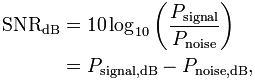
The most significant requirement for a radio receiver is the signal to noise ratio. This is simply the ratio of the signal we want from the sky and the noise from everything else going on in the universe. In truth, from nothing, it's always going to be pretty difficult to get any hard and fast number for the signal to noise ratio. Notwithstanding, it's the thing you want to know most.

The basic problem is that of the surrounding environment. If you try and operate the receiver in a built up area or near to a CRT television, the signal to noise ratio is going to be much worse, than if the radio is at the top of a tall antenna mast, in isolation, in the middle of the field. This is primarily because both the environment, and the quality of the radio design will contribute to the noise. These factors are completely independent of the transmitter. If the noise is bigger than the signal then it's not possible to receive.

Set against this fairly negative view, is the idea that the transmitter sets a definite signal power. Also that the receiver can be both sensitive and selective. If the noise is fixed, and the transmitter increases it's power level then the signal to noise ratio improves, and potentially the transmission can then be received.

Obviously, at the receiver, we have no control over the output power of the transmitter. We have to look at other ways to ensure that the signal to noise ratio is sufficient for reception. This is where the sensitivity and selectivity of the receiver become paramount. Selectivity is the ability of the receiver to discriminate between different transmission frequencies. Sensitivity is simply the ability of the receiver to detect a signal at the frequency of interest.

Signal to Noise Ratio (Spectrum)

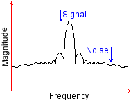
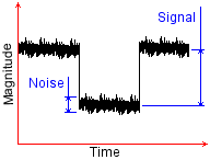
The thing about noise, is that it has a very wide bandwidth. Noise is made up of many things. Included are small things like the noise from space, distant galaxies, the sun, cosmic rays, x-rays and so on. Also included are atmospheric effects, these are things like the magnetosphere (magnetic field of the earth) and effects from the ionosphere. Then there are noise effects from other transmitters, like televisions, other radio stations, car engines and so on. Finally there are the thermal and shot noise effects. These come from the components in the actual radio. They are due to the mechanics of the radio. Shot noise comes from diodes and transistors where electrons are "flicked" across junctions, and thermal noise comes from linear components like resistors where the temperature of the actual device generates pertebations in the basic current.

All of these different effects sum together and produce a wide spectrum of noise. Noise is everywhere to some degree, except perhaps black holes. Fortunately, it doesn't matter to us that radios don't work at all inside black holes! Even more fortunate is that using selectivity, we can choose to ignore most of the noise. The idea here is simple. The more of the noise we can ignore, the bigger our signal is likely to appear, by comparison. Even if the signal to noise ratio in the sky is poor, we can suck the signal we want out of the sky. By improving the selectivity of our receiver, we take a bad signal to noise ratio, and turn it into a good signal to noise ratio.

Sensitivity, perhaps, is a more straightforward concept to grasp. This essentially is the ability of the receiver to detect a small signal. In isolation, it neglects the noise issues, and focusses directly on the issue of the smallest signal that may be received. The relationship between selectivity and sensitivity, is more complex, however. As I perviously described, selectivity can improve sensitivity. With greater selectivity the signal to noise ratio improves, and in effect so does the sensitivity.

The problem is that to reject noise one must use a filter, and most typical filters have an insertion loss. The insertion loss is a measure of the reduction in wanted signal size, for the benefit of a larger (noise rejecting) stopband attenuation. Obviously we can use gain to recover the insertion loss, which is great. We must be careful however, gain stages have a noise figure and if we push the "wanted" signal below the noise floor then the signal will become irrecoverable.

Signal to Noise Ratio (Oscillograph)

As we delve into more detail, we begin to consider how to achieve better selectivity. In practice, the more selectivity we have, the better the sensitivity, right? Well, yes, but it's not quite that simple. For optimum power transfer, electronic circuits must be well matched. If they are not well matched, then power transfer is inefficient. Typically one would use some sort of LC, (Inductor Capacitor) combination to create resonance, and improve selectivity. By adjusting the ratio of inductor to capacitor one may set the specific frequency of resonance. Unfortunately the the Q (selectivity) of the LC combination is mainly influenced by the matching of the LC resonator against the rest of the circuit. By matching the circuit for power transfer, much of the theoretical selectivity of the LC resonator in isolation, is lost. There is a circuit tradeoff between selectivity and gain. The loss in gain is then set against the improvement in sensitivity. Ultimately the selectivity of a resonator will always be limited, but this can be mitigated by isolating and cascading stages of LC resonators.

Overriding all of these issues, is that we can't know what the signal to noise ratio of the signal in the sky actually is. That is to say, we can't know it, until we have a radio to measure it. It's a chicken and egg problem. If we know the signal to noise ratio, and the signal power, we can do some sums and we have a target to hit.

At this stage my approach, was to do some research. I was lucky enough to come across an old Atmel datasheet, for a device, very similar to the EM2S receiver. The Atmel device is now out of production, but it is so similar to the EM2S that I wonder if the EM2S and the Atmel device are the same thing. Irrespective, it provided one, single clue, more useful than all of the other information I was able to research. The old Atmel device was capable of receiving a signal down to 400 nanovolts at its inputs. That is to say, it had 400 nanovolt sensitivity.

NPL MSF Signal Coverage Map

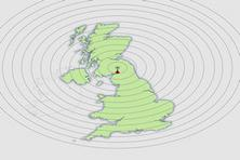
I was also able to establish a spot field strength for MSF at a nominal 1000km distance from the transmitter. This came directly from the NPL website. Stated to be 100 microvolts per meter its importance is rather significant. Currently we don't know what the antenna will look like. We're only considering the receiver electronics. What we can do, however, is make some worst case assumptions. We know that the a radio signal propagates with a power level that is the inverse square of distance. We assume that the antenna is so poor that 100 microvolts per meter translates to 400 nanovolts at the receiver. Then we calculate the maximum signal we expect to see on the receiver, within a kilometre of the transmitter site.

Gradually, and with not a lot to go on, we're beginning to get some numbers to hang things on! I previously suggested that I would be interested in providing AGC on the receiver, and this business of establishing guide numbers is critical to that process. We have to have some means of establishing a Dynamic Range for the receiver.

Previously we discussed calculation of the signal close to the transmitter. To do so, we assumed we would have a poor antenna. Although we don't yet know what the antenna will look like, it's a safe assumption that it will be some kind of Ferrite rod, which is the ideal small antenna solution for LF reception. The problem here is that not all ferrite is the same. There are different grades, and even within those grades there are different levels of performance. Finally, there is almost no data on the composition or performance of ferrite materials.

It could be the case that we actually have a good antenna. In close proximity to the transmitter, the signal could be much larger than we calculate. Perhaps it might saturate the receiver. For my own purposes, it's safe to leave this problem here. From the perspective of a radio receiver one would aim to make it as sensitive as possible. It is very easy to dispose of signal energy, and quite difficult to find it. Most importantly, the antenna gain could change, but the Dynamic Range would remain the same.

If the receiver saturates, it will probably still work assuming the signal to noise ratio is good enough. If the magnitude of the signal is so great that it introduces noise through compression, it's easy enough to solve with a pad in the antenna downlead. Getting that signal back is much harder. The needed performance of the AGC circuit is governed by the geographic size of the continent or country, rather than by component or other physical parameters.

Let's commit to some targets;

These figures have been derived from the considerations above. By no means do these numbers garantee adequate reception. It's more that they represent target design figures. There is undoubtedly a degree of uncertainty, but that is the nature of this kind of receiver. The best test is to build the receiver and see if it works.

Even if we hit these target figures we will have a great deal of difficulty verifying them precisely, since the expensive test kit that would be sensitive enough to measure them is out of reach. Possibly the most important reason for setting them out, is that if the receiver cannot be made to work, we at least have a guide and can make decisions about how to improve the receiver such that it can work.

Despite the lack of expensive resources to verify the receiver performance, for very little money over and above the standard lab equipment, one can determine to "reasonable confidence" that the spec has been met. The signal sizes are very small. A basic signal generator will happily produce a massive 1 volt sinewave. We can easily build low quality resistive pads, and characterise them with a simple multimeter. If we cascade enough of them, we can easily develop a variable voltage between zero and a "nominal" 400nV.

• You may notice that the sensitivity in the spec table has been increased beyond that of the 400nV specification for the referenced Atmel part. This makes allowance for transistors that have practical gains less than the idealised simulation models they represent.
• The selectivity value is probably the second largest unknown. It has been derived more on the basis of what is achievable than desireable. We will be quite fortunate to achieve the desired selectivity.
• The signal to noise ratio is more or less a guess. It is considered at the point of thresholding. It is assumed as the smallest practical received signal level. It is considered here as the worst signal to noise ratio at which reception can be guaranteed.
• Finally, the dynamic range represents the nominal difference between the smallest and largest unsaturated signal levels, prior to the detector circuit. This figure, has been calulated but there is uncertainty. Again, it is a guide and will allow us to assess the performance of the AGC.

Alexanderson Alternator

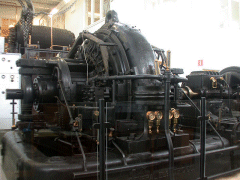
It is unlikely that the receiver will not work at all. One can place almost any electronic system near to the transmitter, and observe reception. A simple metal box ten inches from a 500kW transmitter will literally vibrate. Equally, it is probable that it will not work as well as hoped. Here, where I am developing the receiver, I am nearly 500km from the transmitter. The likely scenario is that diurnal effects will compromise reception at sunrise and sunset. There will almost certainly be periods of time when reception is not possible. At others the signal will be superb. For this reason the first receiver built will be a prototype. In summary we will return to these numbers, knowing broadly if we met the spec in practice. We will also decide on what, if any, improvements are necassary to carry forward into the final receiver.

You will see from other parts of this site that I am an enthusiast for mechanical systems as well as electronic and software ones. Thinking about the vibrating metal box, reminds me that I should make a note about the VLF transmissions in the early days of radio. I find it simply awesome to consider the way that they made these early broadcasts. VLF transmissions have always required relatively high power, and with early valve receivers and limited transmitter sites, it was no different.

The Alexanderson Alternator is a radio frequency alternator such as you would find in a power station or a car running at a much lower frequency. They had few thermionic valves in those days, for a high power application at VLF you don't actually need them. All you need to do is hook up a steam engine!!! Love it!