Receiver Overview

Before we get into circuit details, it's probably going to help if we look at the basic arrangement of a Radio receiver. I already described in the section "Rationale", that I liked the idea of using a TRF for this receiver, so that sets the basic format.

Then, we also have to consider the fairly wide dynamic range that we're hoping to achieve. It's almost certainly going to require that we use some sort of AGC capability. We'll need a detector circuit of some kind. Finally we'll need a way to integrate, or average, the detected signal so that we can threshold the basic radio signal, and pull out a nice clean square wave that we can then use as a digital signal for processing.

The system diagram below shows how all these elements come together;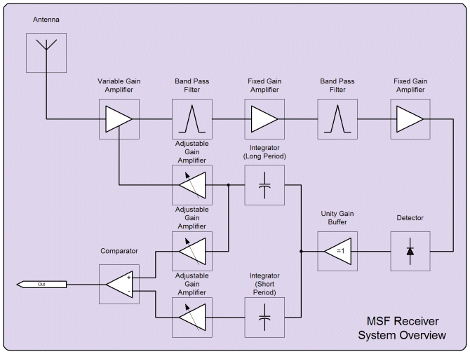

The basic principle of operation here is that the antenna collects the signal. The various amplifiers and filters up to the detector select the MSF signal. Then the detector measures the power of the signal. Since the MSF signal is amplitude modulated, by looking at the power of the signal in respect of time, we can tell if the transmitter is instantaneously on or off. Encoded into these on/off periods is the time signal that we are attempting to recevie.

Remote Transmit Antenna

The electromagnetic induction field

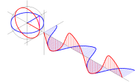
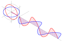
Radio waves are comprised both magnetic and electric field components. The waves themselves propagate from a transmitter which is essentially disturbing the space around it with electrical energy. All electrical conductors (wires) do this, but the transmitter in Anthorn is carefully designed to couple that energy into the space around it very well.

Like ripples in a pool of water the waves radiate in all directions, because there is nothing to absorb them. Instantaneously the radio wave has a given energy, but both the electric and magnetic components of the wave vary in intensity at the frequency of transmission. Although the overall energy from the transmitter is quite high, it must spread out evenly in all directions on the plane of the antenna.

To a very small degree some of the energy is converted into heat as it propagates away from the transmitter, but in general little is lost. What does happen, is that the density of the energy reduces significantly. As the wave moves further from the transmitter site, in all directions, it is spread more and more thinly. Eventually, at great distance from the transmitter the signal energy is so small that it cannot be detected. The signal is still there, but it is smaller than all of the other signals by such a margin as to prevent a machine from measuring it.

At a specific point in space, the radio wave has a quantifiable energy. As it propagates both the electric and magnetic fields oscillate at the frequency of transmission. The actual transmitted energy takes the form of photons (just like light) but the stimulus for those photons are the energetic electrons in the wire of the transmitter antenna. Both photons and electrons have associated electromagnetic fields.

Each, however, may have slightly different relationship between it's electric and magnetic field. Very close to the antenna the induction field, due to the electron motion, has a fixed 90 degree phase relationship between the electric and magnetic field. Further from the antenna the electric and magnetic fields shown in the diagram are in phase. These are due to the propagating photons.

For the photons, the phase relationship of electric and magnetic fields describe the polarisation of the propagating wave. If we stop time, which we can only do in theory, at a given position relative to the transmitter the energy is at least partially electric and partially magnetic, but the relationship depends on the distance from the antenna. Close to the antenna the large induction fields dominate, but decay by the cube of distance. Further away the the radiation field dominates but only decays by the square of distance.

Coupled with diffraction, electromagnetic waves can be steered, and their polarisations controlled. Typically this is done by combining muitliple antennas, collimation, and merely controlling the geometric shape and orientation of an antenna. Typically these actions and operations can control the "free space" signal path to focus energy for optimum transfer and to discriminate and select signals of interest.

The electromagnetic radiation field

It might seem as though I've skipped a rather fundamental detail here. How do the peturbing electrons and fields produce the photons? The question undoubtedly is a good one, and its answer lies in part of science known as Quantum Electrodynamics. I'm afraid I don't have the patience, or probably the brain for that. There is a perfectly functional mathematical explanation that relates the electronics and the photonics.

If you're interested in the Quantum Electrodynamics, there is a truly excellent set of four lectures by Richard Feynman that I would recommend. He's not too heavy on the numbers in that lecture series, and it really does give the best possible view of physics. There's no patronage, but no fear either.

He describes what at the time was a fresh interpretation on Maxwell's Equations, for a probablistic world. There is no longer a need for an electronics engineer to have uncertainty about the wave partical duality. Using what you already know, you can understand that which (perhaps) might not have made sense. More significantly you can see how to take that and begin to apply it not just to electrons and photons, but atomic neuclei, and all fermions and bosons!

Local Receive Antenna

The first component in our system is the receiver antenna. It's simply a coil of wire wrapped around a ferrite rod and positioned in a good location for reception. Because of its iron based fabrication, the field components of the wave pass easily through the ferrite rod, and so nature prefers that path. In particular the coil intercepts the focussed magnetic field component of a radio wave coming from Anthorn. By electomagnetic induction, the field induces an electric current in the coil, and it is this that we subsequently amplify and measure in the receiver.

The trouble with radio waves, is that they are all the same. They are all just electric and magnetic fields. If one were to look only at their strength it would be difficult to tell them apart. It is fortunate then, that they have the property of frequency. This as we saw, is the capability to vary their field energy, as they propagate. The rate at which they do this is the frequency. It is an essential property because using electronic components like capacitors and coils we can select specific frequencies of interest. In electronics it's known as resonance, but in reality, its like a wooden box just beneath the surface of a stream. One makes a box of a particular size. Nature being what it is, only those things that fit the box will collect there. Big twigs are too big to go in. Small twigs go in, but they are washed through. Twigs that fit will get stuck.

Using the ferrite rod, the antenna is attractive to radio waves because of their magnetic field properties. Using resonance with the radio wave's property of frequency, the antenna will have a significant preference for the frequency of interest. In our case it's the MSF signal, but it could have been BBC radio, or even a television signal. Although different signals are encoded by different machines in different ways, all basic radio signals are the same.

Broadly speaking, these two concepts map directly to the sensitivity and selectivity that we have already discussed. The sensitivity is the whole receiver's attractiveness to radio signals. The selectivity, is the ability of the receiver to discriminate between interesting and non interesting signals. Together, they form the basis of radio communication.

Variable Gain Amplifier

Variable Gain Amplifier Response

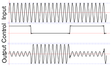
The variable gain amplifier makes allowance for the fact that the receiver can only handle signals of a certain maximum size. In the section on the antenna it was seen that the radio signal can have a wide range of energies at varying distances from the transmitter site. One of the main aims of our transmitter is to amplify the tiny signal that we receive from the transmitter. If we amplify by a fixed amount, then the final signal, although bigger overall, might be bigger or smaller depending on our distance from the transmitter. If the radio signal were very big, the final signal might be too big for use in the receiver. If the radio signal were very small, we may not be able to measure it.

The variable gain amplifier allows us to look at the final signal, and decide if it is too big or too small. In either case, by controlling the gain of the first amplifier we can maintain a consistent signal size throughout the system, irrespective of the power of the incoming signal. The control signal is derived later in the receiver process. Shortly we'll see how that works.

Band Pass Filter

Bandpass Filter Response

The radio uses more than one band pass filter, but they are all identical. When discussing the antenna I mentioned the property of resonance and selectivity. In the antenna resonance was used to pick out the one radio signal of interest to us, the MSF broadcast. Here, we use the bandpass filter in the same way. After the first amplifier, the variable gain, the signal is much bigger and stronger. It's potentially not as big as we'd like or need, so we'll need to use more amplification. The problem with all of this amplification, is that it's not very frequency selective.

The selectivity of the antenna is not as good as we would like. Although it has a preference for signals at the frequency of interest to us, When we make the signal from the antenna bigger we make both the smaller unwanted signals bigger, along with the signal that we want. This additional bandpass filter is used to make the signals that we don't want, smaller again.

In the diagram there are multiple stages of amplification and filtering. At each stage, we attempt to make the signal we want bigger relative to the unwanted ones. This is the most important aspect of the capability to receive a radio signal.

Detector / Buffer / Integrator

Detector Response

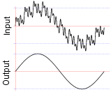
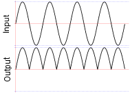
Up until now all of the signals that the receiver has worked on, have been sine wave representations of the of the original radio signal the antenna pulled out of the sky. Using amplification and filtering we have made the signal that we wanted, the biggest of all, and rejected unwanted signals. Usign the amplification the radio signal is now easily measurable using ordinary electronic components.

The information encoded in the radio signal comes in the form of a variable amplitude. In the case of MSF, the modulation is 100%. Sometimes the transmitter is off, sometimes it is on. We need a way to work out this on/off status. In general terms one might think it easy to simply measure the size of the sine wave. In practice it is rather more difficult because of the way sine waves behave.

In a digital environment it is quite straightforward to repeatedly measure the instantaneous size of a sine wave. By taking the biggest measured signal and subtracting the smallest measured signal one quickly has the amplitude of the sine wave. At this stage we don't want to increase the complexity of the receiver by sampling the signal and introducing a microprocessor. We must use analogue techniques.

Pretty nearly the only useful analogue technique here is averaging, or integration. Typically, the idea is that a capacitor is used to store charge over time. Although the signal is varying, we can set up the capacitor such that it will charge and discharge at a given rate, for a given applied voltage. In essence, when we place a rough bumpy signal onto the integrator, we'll get a smooth averaged signal out. It sounds ideal, we could apply our sinewave, and it would tell us the average value.

Integrator Response

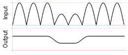
The trouble is that the average value of a sinewave, is zero, or at least the value of the offset applied. It's just the way things work. Because the capacitor lets the variable signal components through, it can't usefully average the amplitude of the sine wave, only it's offset. The positive going half cycles of the sine wave cancel out the negative half cycles, adf the average is zero.

This then, is the function of the detector. By using a diode, one can strip either the positive or negative half cycles from the signal. Suddenly, the average of the discontinuous waveform, is the sum of the magnitude of the sine wave, and it's offset. In our receiver, we'll use full wave rectification, and here I've discussed half wave rectification. It doesn't matter, the principle is the same. The average of a discontinuous signal is the sum of the offset and some proportin of the amplituide depending on it's shape.

By ensuring that the offset is near zero, and because we are sure that the shape of the waveform will be consistent, the average value of the waveform, calculated in the integrator, is directly related to the amplitude of the sinewave applied to the detector.

The buffer stage is used because the integrator uses a capacitor. The output of the detector is a comparitively weak signal, and the detector uses internal feedback in order to produce an accurately shaped voltage signal. Also we need two integrators that average the amplitude of the radio signal, as I'll discuss. If we simply connected the integrators and the detector together, the integrators would interfere with each other, and both would affect the quality of the signal produced by the detector.

The buffer is simply an amplifier, but it has a gain of one. This means that the voltage signal applied to it's input is the same as the voltage that it produces on the output. The buffer amplifier isolates the various functions such that they may not interfere with each other. Overall, however, it has no computational effect on the signal.

Adjustable Gain Amplifiers

There are a range of adjustable gain amplifiers. The idea of them being adjustable does not necassarily mean they are adjustable in the final circuit. It is merely important that their specific gains are measured, considered and set. Unlike the variable gain amplifiers, the adjustable gain amplifiers do not change their gains once set. Certainly, it is important they do not change whilst the radio is receiving. The adjustable gain amplifiers, are also unlike the fixed gain amplifiers. There the exact gain is not particularly known or important, just so long as it is big enough.

The variable gain amplifiers produce three gritical signals in the system. Probably the most important is the AGC signal. The agc signal is that which controls the gain of the variable gain amplifier. The AGC signal is derived from the long integrator average signal. The purpose of the long average is to indicate the power of the signal over a longer timescale than any interruption of the radio signal due to information encoding. The important point here, is that the long average is a slowly changing smooth signal.

The top adjustable gain amplifer scales the long average, for the gain control input to the variable gain amplifier. At the beginning we described how this amplifier maintains a consistent signal size throughout the receiver. Now we can see how this is achieved through feedback. As the input signal grows, the long average also grows. Through the adjustable scaling amplifier, the ACG signal grows, and this reduces the gain of the variable gain amplifer. In turn this reduces the size of the signal in the system. In practice the overall gain of the signal path varies with the size of the input signal. Notably this control does not produce oscillation on it's own. The only reason is that the averaging function is slow enough that the feedback loop is stable.

Comparator

The remaining two adjustable gain amplifiers scale the long average, the short average and bring them together in the comparator. The aim of the short average is simply to remove transients, noise and any remnants of the original rectified sine wave - the radio frequency signal. The short average intentionally contains an indication of the breaks in transmission - the amplitude codes in the signal. By comparing the fast average and the slow average in an appropriately scaled way, one can produce a nice clean square wave which indicates when the transmitter is switched on and off.

This square wave, probably by design, closely mimics the form of RS232. Although the signal levels from the comparator are not RS232, the timing of the encoding is so close that a level shifted version of this signal can be fed into the serial port of an ordinary computer. Once inside the computer, individual bits can be extracted and stored. Once verified, these can be used to establish the exact time and date.