The linear mathematical operators - Add and Subtract

Ohms Law

On this page, I'm going to cover what I would describe as the linear mathematical operators. This fits both of the add and subtract operators, and I refer to it as linear since if you connect both inputs together and vary them, then outputs when plotted against the inputs trace out a nice straight line. Clearly, if you did the same with a multiplier, then you wouldn't get a straight line! I'll cover the multiply operator on a later page.

Using Op-Amps for mathematical operators is largely an obsolete science now. Once, before the advent of the digital computer, the analogue computer was the only available technique. Probably the most important benefit of such a technique, even today, is propagation delay. Although computer technologies are more precise, and can provide phenomenal computation bandwidth, they are generally subject to significant pipeline delays. With a simple amplifier circuit, one can achieve reasonable accuracy with very low latency, and little design overhead.

The summing amplifier

The drawing below shows the general configuration of a summing amplifier. Probably the best comparison with what I've described thus far is the inverting amplifier. In fact the summing configuration is pretty easy to think about. Like the inverting configuration the inputs generally are connected to the inverting input of the amplifier. If you remember back to the inverting amplifier configuration, you'll remember how two resistors governed the gain of the amplifier.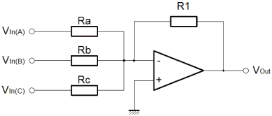

At the inverting input, the voltage was controlled by the feedback loop, to match the potential at the non-inverting input. Since the non-inverting input was connected to ground the inverting input too was maintained at ground potential. This had an important consequence; the current in both resistors was the same.

Here, the arrangement is the same, but there are more resistors, and more inputs. The only real difference is that more inputs feed the same inverting input virtual ground. The feedback resistor still maintains a minimal difference between the Op-Amp inputs. The net result is that the feedback resistor carries the sum of the currents supplied by the various inputs. The only thing to notice is that although the inputs are added, the configuration of the amplifier causes the sum to be negated. To achieve a true sum, one would need to add an inverting amplifier after the summing amplifier.

The function below shows how to calculate the overall output. As you can see this is a multivariable problem, so the utility of this actual function is limited. Its usefulness really lies in demonstrating the behaviour of the circuit, and I've included it here for completeness.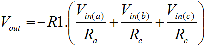

Clearly with the feedback resistor (R1), one can control the overall gain. With each of the input resistors (Ra-c), one can control the relative weights for each of the inputs. An obvious application for this kind of circuit is a simple audio mixer. Each channel of audio can be fed into the inputs, and then by replacing the fixed resistors with potentiometers, one can mix the audio, much like a mixing desk.

In an attempt to mitigate the previously described lack of usefulness, I've used an assumption that all of the inputs are connected together. Obviously all of the inputs are weighted according to their input resistors. To get a function that looks something like a gain, without a reference to the input resistors the assumption has to be made. The function is shown below;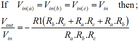

The idea that all of the inputs are at the same potential is not very realistic; the whole purpose of the summing amplifier is to sum a variety signals with different information in them. Previously I showed how to calculate the output of the summing amplifier for given inputs. Now I've shown how to calculate the overall gain of the summing amplifier. The trouble is that there is no easy way to express both at the same time. One must use two different techniques to evaluate the overall performance of the amplifier. The utility of the combined input gain approach is that it gives a way to express the dynamic range of the inputs as compared with the output.

The idea of dynamic range here is important. Dynamic range, expresses the ratio of the smallest and largest measurable signals. Although we don't know the magnitude of the smallest measurable signal, it is unimportant, since it will be (more or less) the same for a given Op-Amp, and we won't have a high degree of control over it. By contrast, the largest signal we have a great degree of control over. In general terms it is governed by the voltage on the supply rails we choose for our circuit.

If we chose plus/minus 5v supply rails for our circuit, then the three input signals might nominally swing from plus to minus 4 volts. When we add these signals we could potentially end up with a maximum and minimum output of plus or minus 12 volts. This would violate the power supply voltages, and the amplifier would saturate and distort. For this reason, the gain function is useful, since it allows us to check that the inputs cannot cause the output to exceed its capability. Another similar and important consequence of this reasoning is that the sum of the signals increases the required dynamic range of the output. In order to realise a practical summing circuit, we cannot avoid wasting some of the dynamic range in the inputs.

It is possible to trade the dynamic range available at the output between the inputs. Here, the problem is one of magnitude. Those inputs with less available dynamic range will be smaller at the output. If a scheme can be provided which constrains the inputs and feedback to an output which may not saturate, then one has a system which is very flexible. Typically such a scheme is the preserve of the digital domain where the additional complexity has a limited physical and cost overhead. Normally with an analogue summing circuit one would expect the inputs to have equal weighting, such that if there are "N" inputs each with similar dynamic range "M" then the output dynamic range will be "M divided by N".

The difference amplifier

The final linear amplifier I'll show here is the difference amplifier. Clearly it is possible to achieve a subtraction mathematical operator using the circuits already described. Since we know how to add signals, and we also know how to invert them, we can combine the inverter and the summer, to perform subtraction. Here, we take a different approach. By using the inverting and non inverting inputs of the amplifier, we can perform subtraction with a single amplifier.

The diagram below shows the difference configuration of the Op-Amp. In practice it is similar to the inverting configuration. In the inverting configuration, we used the ratio of the input and feedback resistors to govern the gain of the amplifier. We knew that the potential at the inverting input of the amplifier had to match that of the non-inverting input. In that case the non-inverting input was tied to ground or zero. Here, all we are doing is additionally varying the potential at the non-inverting input. Now, the potential at the inverting input must follow a moving target. The output is a function of the Vin(-) plus Vin(+).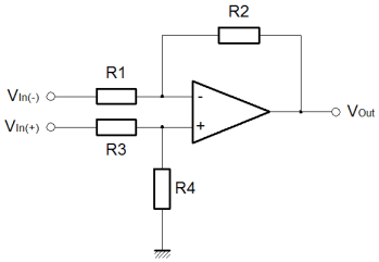

Like the summing amplifier, I've shown the equation that describes the output of the amplifier, below. As before the equation is of limited use since it is a multivariable problem. Certainly, it represents a good starting point for analysis and re-arrangement for any application you may have for the difference amplifier.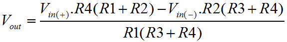

To round out the deal, I've made the assumption that the inputs are the same, in order to allow calculation of a gain, which is more useful. The equation is shown below. Just as before with the summing amplifier, all the same thinking about dynamic range applies. The big change here is clearly that one signal is being subtracted from the other. This might lead to the conclusion that the relationship between the input and output dynamic range be improved. In actual fact this is no more or less the case than it was before. Just like an input to the summer could have been inverted, or negated, so could it here.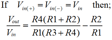

If you click on the equations you'll find the derivations for the functions presented here. In addition, there is a third derivation that I did. If you remember back to the simple inverting and non-inverting configurations I briefly looked at the effect of the actual Op-Amp gain on the performance of the circuit. The third derivation, not shown, does this for the difference amplifier. This may or may not be useful, but it's included there if you need it.

The generic linear operator

To try and express this issue of trading the dynamic range more certainly, consider the circuit below. This circuit allows the sum and difference of a range of signals. Multiple values are added, and multiple values are subtracted. All of this is achieved with a single Op-Amp. The idea in the diagram should seem straightforward by now.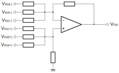

In the summing configuration we increased the number of inputs to the inverting amplifier, such that we could add the inputs together. Although we calculated the sum of the input, the output was inverted. Now we're dealing with the parts to be added to the output on the non-inverting input of the amplifier, the node that represented the summing junction in the summing amplifier is now the node that represents the sum of the parts to subtract. In the summing amplifier, the implicit inversion was unwanted. Now we can turn it to our advantage.

I've not included any maths for the generic linear operator. I'll leave that for you to do. The important thing to realise from the perspective of these articles is that we are moving more towards the Op-Amp as the "little triangle" it really is. Once you can see how to use it in a few simple configurations, it becomes easier and easier to invent your own configurations, by tacking components around it to suit the application.